SWAN procedural example#
In this notebook we will use the SWAN Components and data objects to define a SWAN workspace
[1]:
%load_ext autoreload
%autoreload 2

import shutil
from pathlib import Path
import numpy as np
import xarray as xr
import matplotlib.pyplot as plt
import cmocean
from cartopy import crs as ccrs

import warnings
warnings.filterwarnings("ignore")
Workspace basepath#
[2]:
workdir = Path("example_procedural")
shutil.rmtree(workdir, ignore_errors=True)
workdir.mkdir()
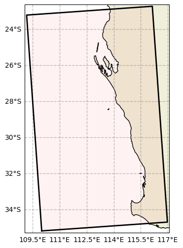
Model Grid#
[3]:
from rompy.swan.grid import SwanGrid

grid = SwanGrid(
    x0=110.0,
    y0=-35.2,
    rot=4.0,
    dx=0.5,
    dy=0.5,
    nx=15,
    ny=25,
)

fig, ax = grid.plot(fscale=6)
Work with existing data#
We will work with subsets of global bathymetry from Gebco, winds from ERA5 and spectral boundary from Oceanum available in Rompy. Some dummy interpolation routine is used to exemplify how existing xarray datasources could be processed and then provided to rompy to define the model config
[4]:
from rompy.core.time import TimeRange
from rompy.core.types import DatasetCoords
from rompy.core.source import SourceDataset
from rompy.swan.data import SwanDataGrid
from rompy.swan.boundary import Boundnest1

projection = ccrs.PlateCarree()
[5]:
def my_fancy_interpolation(
    dset: xr.Dataset,
    grid: SwanGrid,
    coords: DatasetCoords,
    buffer: float = 0.0,
) -> xr.Dataset:
    """Dummy interpolation function."""
    x0, y0, x1, y1 = grid.bbox(buffer)
    xarr = np.arange(x0, x1+grid.dx, grid.dx)
    yarr = np.arange(y0, y1+grid.dy, grid.dy)
    return dset.interp(**{coords.x: xarr, coords.y: yarr})
[6]:
DATADIR = Path("../../tests/data")
display(sorted(DATADIR.glob("*")))

gebco = xr.open_dataset(DATADIR / "gebco-1deg.nc")
era5 = xr.open_dataset(DATADIR / "era5-20230101.nc")
oceanum = xr.open_dataset(DATADIR / "aus-20230101.nc")
[PosixPath('../../tests/data/aus-20230101.nc'),
 PosixPath('../../tests/data/catalog.yaml'),
 PosixPath('../../tests/data/era5-20230101.nc'),
 PosixPath('../../tests/data/gebco-1deg.nc')]
Times#
[7]:
# Define a time object to run the model using the time range from ERA5 dataset

start, end = era5.time.to_index()[[0, -1]]
times = TimeRange(start=start, end=end, interval="1h")
times
[7]:
TimeRange(start=Timestamp('2023-01-01 00:00:00'), end=Timestamp('2023-01-02 00:00:00'), duration=Timedelta('1 days 00:00:00'), interval=datetime.timedelta(seconds=3600), include_end=True)
Bathy#
[8]:
# Display the GEBCO dataset

display(gebco)
p = gebco.elevation.plot(figsize=(10, 5), cmap=cmocean.cm.topo)
<xarray.Dataset> Size: 526kB
Dimensions:    (lat: 181, lon: 360)
Coordinates:
  * lon        (lon) int64 3kB 0 1 2 3 4 5 6 7 ... 353 354 355 356 357 358 359
  * lat        (lat) int64 1kB -90 -89 -88 -87 -86 -85 -84 ... 85 86 87 88 89 90
Data variables:
    elevation  (lat, lon) float64 521kB ...
Attributes:
    title:    Subset of the GEBCO 2020 grid for testing purposes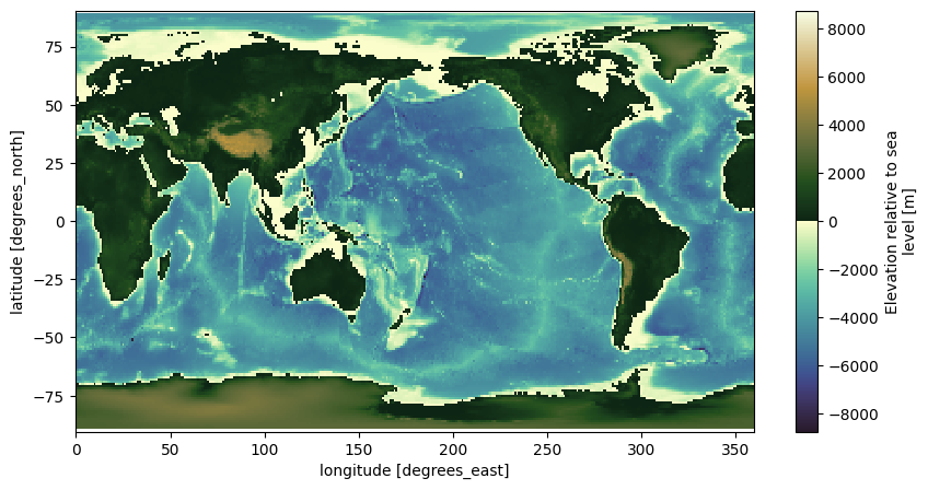
[9]:
# Process gebco into the model bathy

dset = my_fancy_interpolation(gebco, grid, DatasetCoords(x="lon", y="lat"), buffer=1.0)
dset
[9]:
<xarray.Dataset> Size: 5kB
Dimensions:    (lat: 30, lon: 21)
Coordinates:
  * lon        (lon) float64 168B 108.2 108.7 109.2 109.7 ... 117.2 117.7 118.2
  * lat        (lat) float64 240B -36.2 -35.7 -35.2 -34.7 ... -22.7 -22.2 -21.7
Data variables:
    elevation  (lat, lon) float64 5kB -5.443e+03 -5.552e+03 ... 333.9 346.7
Attributes: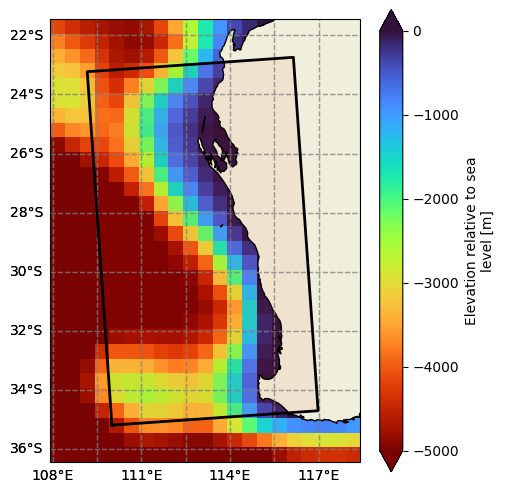
title: Subset of the GEBCO 2020 grid for testing purposes[10]:
# Create and plot the data instance. This object will be provided to the SWAN Config through the DataInterface

bottom = SwanDataGrid(
    var="bottom",
    source=SourceDataset(obj=dset),
    z1="elevation",
    fac=-1,
    coords={"x": "lon", "y": "lat"},
    crop_data=False, # So data isn't cropped to model grid inside SwanConfig
)

fig, ax = bottom.plot(param="elevation", vmin=-5000, vmax=0, cmap="turbo_r", figsize=(5, 6))
grid.plot(ax=ax);
Winds#
[11]:
# Display the ERA dataset

display(era5)

fu = era5.u10.plot(col="time", figsize=(15, 1.5), subplot_kws={"projection": projection}, cbar_kwargs={"label": "u (m/s)"})
fv = era5.v10.plot(col="time", figsize=(15, 1.5), subplot_kws={"projection": projection}, cbar_kwargs={"label": "v (m/s)"})
for f in [fu, fv]:
    f.map(lambda: plt.gca().coastlines())
<xarray.Dataset> Size: 214kB
Dimensions:    (latitude: 37, longitude: 72, time: 5)
Coordinates:
  * latitude   (latitude) float32 148B 90.0 85.0 80.0 75.0 ... -80.0 -85.0 -90.0
  * longitude  (longitude) float32 288B 0.0 5.0 10.0 15.0 ... 345.0 350.0 355.0
  * time       (time) datetime64[ns] 40B 2023-01-01 ... 2023-01-02
Data variables:
    u10        (time, latitude, longitude) float64 107kB ...
    v10        (time, latitude, longitude) float64 107kB ...
Attributes:
    Conventions:  CF-1.6
    history:      2023-06-10 00:03:38 GMT by grib_to_netcdf-2.25.1: /opt/ecmw...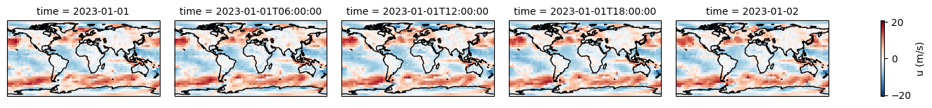
[12]:
# Process it into the model forcing

dset = my_fancy_interpolation(era5, grid, DatasetCoords(x="longitude", y="latitude"), buffer=1.0)
dset
[12]:
<xarray.Dataset> Size: 51kB
Dimensions:    (time: 5, latitude: 30, longitude: 21)
Coordinates:
  * time       (time) datetime64[ns] 40B 2023-01-01 ... 2023-01-02
  * longitude  (longitude) float64 168B 108.2 108.7 109.2 ... 117.2 117.7 118.2
  * latitude   (latitude) float64 240B -36.2 -35.7 -35.2 ... -22.7 -22.2 -21.7
Data variables:
    u10        (time, latitude, longitude) float64 25kB 3.054 3.084 ... 1.339
    v10        (time, latitude, longitude) float64 25kB 4.884 4.951 ... 0.9003
Attributes:
    Conventions:  CF-1.6
history: 2023-06-10 00:03:38 GMT by grib_to_netcdf-2.25.1: /opt/ecmw...[13]:
# ERA5 has Latitude in reverse order, use filter to reverse it

from rompy.core.filters import Filter
[14]:
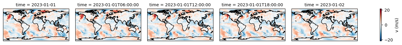
# Create and plot the data instance. This object will be provided to the SWAN Config through the DataInterface

wind = SwanDataGrid(
    var="wind",
    source=SourceDataset(obj=dset),
    z1="u10",
    z2="v10",
    coords={"x": "longitude", "y": "latitude"},
    crop_data=False, # So data isn't cropped to model grid inside SwanConfig
    filter=Filter(sort=dict(coords=["latitude"]))
)

fig, ax = wind.plot(param="u10", isel={"time": 0}, vmin=-5, vmax=5, cmap="RdBu_r", figsize=(5, 6))
grid.plot(ax=ax);
Boundary#
[15]:
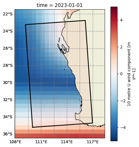
# Open and check the test spectra dataset

display(oceanum)

fig, ax = plt.subplots(figsize=(10, 5), subplot_kw={"projection": projection})
c = oceanum.isel(time=[0]).spec.hs()
p = ax.scatter(oceanum.lon, oceanum.lat, s=6, c=c, cmap="turbo", vmin=0, vmax=4)
ax.set_title(c.time.to_index().to_pydatetime()[0])
plt.colorbar(p, label=f"Hs (m)")
ax.coastlines()
grid.plot(ax=ax);
<xarray.Dataset> Size: 1MB
Dimensions:  (time: 5, site: 412, freq: 11, dir: 8)
Coordinates:
  * time     (time) datetime64[ns] 40B 2023-01-01 ... 2023-01-02
  * site     (site) int64 3kB 0 4 8 12 16 20 ... 1624 1628 1632 1636 1640 1644
  * freq     (freq) float32 44B 0.05417 0.05959 0.06555 ... 0.1161 0.1277 0.1405
  * dir      (dir) float32 32B 0.0 45.0 90.0 135.0 180.0 225.0 270.0 315.0
Data variables:
    lon      (site) float32 2kB ...
    lat      (site) float32 2kB ...
    efth     (time, site, freq, dir) float64 1MB ...
    dpt      (time, site) float32 8kB ...
    wspd     (time, site) float32 8kB ...
    wdir     (time, site) float32 8kB ...
Attributes: (12/16)
    product_name:           ww3.all_spec.nc
    area:                   Global 0.5 x 0.5 degree
    data_type:              OCO spectra 2D
    format_version:         1.1
    southernmost_latitude:  n/a
    northernmost_latitude:  n/a
    ...                     ...
    minimum_altitude:       n/a
    maximum_altitude:       n/a
    altitude_resolution:    n/a
    start_date:             2023-01-01 00:00:00
    stop_date:              2023-02-01 00:00:00
    field_type:             3-hourly
[16]:
# Create the boundary instance. This object will be provided to the SWAN Config through the BoundaryInterface

boundary_from_data = Boundnest1(
    id="westaus",
    source=SourceDataset(obj=oceanum),
    sel_method="idw",
    sel_method_kwargs={"tolerance": 4}, # points are sparse around the offshore boundary so make sure tolerance is appropriate
)
[17]:
# Generate the boundary data and plot them to check.
# This isn't necessary but it is useful for checking the generated boundary look okay

# Generate the boundary data
outfile, cmd = boundary_from_data.get(destdir=workdir, grid=grid, time=times)

# Read the boundary data into an xarray dataset
from wavespectra import read_swan

ds = read_swan(outfile)
display(ds)

# Plot the boundary data alongside the source dataset and the model grid
fig, ax = plt.subplots(figsize=(10, 5), subplot_kw={"projection": projection})

# Source dataset
c = oceanum.isel(time=[0]).spec.hs()
p = ax.scatter(oceanum.lon, oceanum.lat, s=20, c=c, marker="v", cmap="turbo", vmin=0, vmax=4)

# Generated boundary dataset
c = ds.isel(time=[0]).spec.hs()
p = ax.scatter(ds.lon, ds.lat, s=50, c=c, cmap="turbo", edgecolors="0.5", vmin=0, vmax=4)

# Model grid
grid.plot(ax=ax)

# Axis settings
ax.set_title(c.time.to_index().to_pydatetime()[0])
plt.colorbar(p, label=f"Hs (m)")
ax.coastlines()
ax.set_extent([ds.lon.min()-3, ds.lon.max()+3, ds.lat.min()-3, ds.lat.max()+3])
<xarray.Dataset> Size: 273kB
Dimensions:  (time: 5, site: 77, freq: 11, dir: 8)
Coordinates:
  * time     (time) datetime64[ns] 40B 2023-01-01 ... 2023-01-02
  * site     (site) int64 616B 1 2 3 4 5 6 7 8 9 ... 69 70 71 72 73 74 75 76 77
  * freq     (freq) float64 88B 0.05417 0.05959 0.06555 ... 0.1161 0.1277 0.1405
  * dir      (dir) float64 64B 0.0 45.0 90.0 135.0 180.0 225.0 270.0 315.0
Data variables:
    efth     (time, site, freq, dir) float64 271kB 0.0 0.0 ... 5.238e-05
    lat      (site) float64 616B -35.2 -35.17 -35.13 -35.1 ... -34.2 -34.7 -35.2
    lon      (site) float64 616B 110.0 110.5 111.0 111.5 ... 109.9 110.0 110.0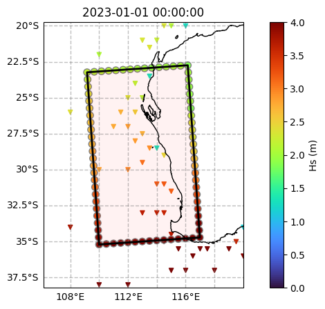
SWAN components#
SWAN commands can be fully prescribed using what we define as “Components”. Components are pydantic objects that describe the different sets of command instruction in SWAN with fields that matching command options and a render() method that returns the string to render in the INPUT command file.
The SwanConfigComponents config class takes the components as fields organised as “group” components, a collection of individual components that are defined together and validated for consistency. These groups are structured similarly to the main groups of SWAN commands as defined by the subsections in Chapter 4 of the user manual.
[18]:
from rompy.swan.config import SwanConfigComponents

SwanConfigComponents?
Init signature:
SwanConfigComponents(
    *,
    model_type: Literal['swanconfig', 'SWANCONFIG'] = 'swanconfig',
    template: str = '/source/csiro/rompy/rompy/templates/swancomp',
    checkout: Optional[str] = 'main',
    cgrid: Union[rompy.swan.components.cgrid.REGULAR, rompy.swan.components.cgrid.CURVILINEAR, rompy.swan.components.cgrid.UNSTRUCTURED],
    startup: Optional[Annotated[rompy.swan.components.group.STARTUP, FieldInfo(annotation=NoneType, required=True, description='Startup components')]] = None,
    inpgrid: Optional[Annotated[Union[rompy.swan.components.group.INPGRIDS, rompy.swan.interface.DataInterface], FieldInfo(annotation=NoneType, required=True, description='Input grid components', discriminator='model_type')]] = None,
    boundary: Optional[Annotated[Union[rompy.swan.components.boundary.BOUNDSPEC, rompy.swan.components.boundary.BOUNDNEST1, rompy.swan.components.boundary.BOUNDNEST2, rompy.swan.components.boundary.BOUNDNEST3, rompy.swan.interface.BoundaryInterface], FieldInfo(annotation=NoneType, required=True, description='Boundary component', discriminator='model_type')]] = None,
    initial: Optional[Annotated[rompy.swan.components.boundary.INITIAL, FieldInfo(annotation=NoneType, required=True, description='Initial component')]] = None,
    physics: Optional[Annotated[rompy.swan.components.group.PHYSICS, FieldInfo(annotation=NoneType, required=True, description='Physics components')]] = None,
    prop: Optional[Annotated[rompy.swan.components.numerics.PROP, FieldInfo(annotation=NoneType, required=True, description='Propagation components')]] = None,
    numeric: Optional[Annotated[rompy.swan.components.numerics.NUMERIC, FieldInfo(annotation=NoneType, required=True, description='Numerics components')]] = None,
    output: Optional[Annotated[rompy.swan.components.group.OUTPUT, FieldInfo(annotation=NoneType, required=True, description='Output components')]] = None,
    lockup: Optional[Annotated[rompy.swan.components.group.LOCKUP, FieldInfo(annotation=NoneType, required=True, description='Output components')]] = None,
    **extra_data: Any,
) -> None
Docstring:
SWAN config class.

TODO: Combine boundary and inpgrid into a single input type.

Note
----
The `cgrid` is the only required field since it is used to define the swan grid
object which is passed to other components.
Init docstring:
Create a new model by parsing and validating input data from keyword arguments.

Raises [`ValidationError`][pydantic_core.ValidationError] if the input data cannot be
validated to form a valid model.

`self` is explicitly positional-only to allow `self` as a field name.
File:           /source/csiro/rompy/rompy/swan/config.py
Type:           ModelMetaclass
Subclasses:
CGRID#
[19]:
from rompy.swan.components.cgrid import REGULAR
from rompy.swan.subcomponents.readgrid import GRIDREGULAR
from rompy.swan.subcomponents.spectrum import SPECTRUM

cgrid = REGULAR(
    grid=GRIDREGULAR(
        xp=grid.x0,
        yp=grid.y0,
        alp=grid.rot,
        xlen=grid.xlen,
        ylen=grid.ylen,
        mx=grid.nx -1,
        my=grid.ny -1,
    ),
    spectrum=SPECTRUM(
        mdc=36,
        flow=0.04,
        fhigh=1.0,
    ),
)

print(cgrid.render())
CGRID REGULAR xpc=110.0 ypc=-35.2 alpc=4.0 xlenc=7.0 ylenc=12.0 mxc=14 myc=24 CIRCLE mdc=36 flow=0.04 fhigh=1.0
Startup#
[20]:
from rompy.swan.components.group import STARTUP
from rompy.swan.components.startup import PROJECT, SET, MODE, COORDINATES
from rompy.swan.subcomponents.startup import SPHERICAL

project = PROJECT(
    name="Test procedural",
    nr="run1",
    title1="Procedural definition of a Swan config with rompy",
)

set = SET(level=0.0, depmin=0.05, direction_convention="nautical")

mode = MODE(kind="nonstationary", dim="twodimensional")

coordinates = COORDINATES(kind=SPHERICAL())

startup = STARTUP(
    project=project,
    set=set,
    mode=mode,
    coordinates=coordinates,
)

print(startup.render())
PROJECT name='Test procedural' nr='run1' title1='Procedural definition of a Swan config with rompy'

SET level=0.0 depmin=0.05 NAUTICAL

MODE NONSTATIONARY TWODIMENSIONAL

COORDINATES SPHERICAL CCM
Input grids#
We will prescribe input grids from our previously defined SwanDataGrid objects using the DataInterface object. This object is used by SwanConfigComponents as an interface to pass around times and grids between model and data objects, create model input times and generate consistent CMD instructions.
[21]:
from rompy.swan.interface import DataInterface

inpgrid = DataInterface(
    bottom=bottom,
    input=[wind],
)

inpgrid
[21]:
DataInterface(model_type='data_interface', bottom=SwanDataGrid(model_type='data_grid', id='data', source=SourceDataset(model_type='dataset', obj=<xarray.Dataset> Size: 5kB
Dimensions:    (lat: 30, lon: 21)
Coordinates:
  * lon        (lon) float64 168B 108.2 108.7 109.2 109.7 ... 117.2 117.7 118.2
  * lat        (lat) float64 240B -36.2 -35.7 -35.2 -34.7 ... -22.7 -22.2 -21.7
Data variables:
    elevation  (lat, lon) float64 5kB -5.443e+03 -5.552e+03 ... 333.9 346.7
Attributes:
    title:    Subset of the GEBCO 2020 grid for testing purposes), link=False, filter=Filter(sort={}, subset={}, crop={}, timenorm={}, rename={}, derived={}), variables=['elevation'], coords=DatasetCoords(t='time', x='lon', y='lat', z='depth', s='site'), crop_data=False, buffer=0.0, time_buffer=[0, 0], z1='elevation', z2=None, var=<GridOptions.BOTTOM: 'bottom'>, fac=-1.0), input=[SwanDataGrid(model_type='data_grid', id='data', source=SourceDataset(model_type='dataset', obj=<xarray.Dataset> Size: 51kB
Dimensions:    (time: 5, latitude: 30, longitude: 21)
Coordinates:
  * time       (time) datetime64[ns] 40B 2023-01-01 ... 2023-01-02
  * longitude  (longitude) float64 168B 108.2 108.7 109.2 ... 117.2 117.7 118.2
  * latitude   (latitude) float64 240B -36.2 -35.7 -35.2 ... -22.7 -22.2 -21.7
Data variables:
    u10        (time, latitude, longitude) float64 25kB 3.054 3.084 ... 1.339
    v10        (time, latitude, longitude) float64 25kB 4.884 4.951 ... 0.9003
Attributes:
    Conventions:  CF-1.6
    history:      2023-06-10 00:03:38 GMT by grib_to_netcdf-2.25.1: /opt/ecmw...), link=False, filter=Filter(sort={}, subset={}, crop={}, timenorm={}, rename={}, derived={}), variables=['u10', 'v10'], coords=DatasetCoords(t='time', x='longitude', y='latitude', z='depth', s='site'), crop_data=False, buffer=0.0, time_buffer=[0, 0], z1='u10', z2='v10', var=<GridOptions.WIND: 'wind'>, fac=1.0)])
Boundary#
Boundary can be defined either from a SWAN boundary component or using the BoundaryInterface class which works in an analogous way to DataInterface.
Below we define a pure parametric boundary using the BOUNDSPEC component just to demonstrate it:
[22]:
from rompy.swan.components.boundary import  BOUNDSPEC
from rompy.swan.subcomponents.boundary import SIDE, CONSTANTPAR
from rompy.swan.subcomponents.spectrum import SHAPESPEC, JONSWAP

shape = JONSWAP(gamma=3.3)

shapespec = SHAPESPEC(shape=shape, per_type="peak", dspr_type="degrees")

location = SIDE(side="west", direction="ccw")

data = CONSTANTPAR(hs=2.0, per=12.0, dir=255.0, dd=25.0)

boundary_parametric = BOUNDSPEC(shapespec=shapespec, location=location, data=data)

print(boundary_parametric.render())
BOUND SHAPESPEC JONSWAP gamma=3.3 PEAK DSPR DEGREES
BOUNDSPEC SIDE WEST CCW CONSTANT PAR hs=2.0 per=12.0 dir=255.0 dd=25.0
And here we define boundary from the data using the BoundaryInterface object which interfaces that with the time and grid objects within SwanConfig:
[23]:
from rompy.swan.interface import BoundaryInterface

boundary_interface = BoundaryInterface(
    kind=boundary_from_data
)

boundary_interface
[23]:
BoundaryInterface(model_type='boundary_interface', kind=Boundnest1(model_type='boundnest1', id='westaus', source=SourceDataset(model_type='dataset', obj=<xarray.Dataset> Size: 1MB
Dimensions:  (time: 5, site: 412, freq: 11, dir: 8)
Coordinates:
  * time     (time) datetime64[ns] 40B 2023-01-01 ... 2023-01-02
  * site     (site) int64 3kB 0 4 8 12 16 20 ... 1624 1628 1632 1636 1640 1644
  * freq     (freq) float32 44B 0.05417 0.05959 0.06555 ... 0.1161 0.1277 0.1405
  * dir      (dir) float32 32B 0.0 45.0 90.0 135.0 180.0 225.0 270.0 315.0
Data variables:
    lon      (site) float32 2kB 108.0 108.0 108.0 108.0 ... 157.0 157.0 157.0
    lat      (site) float32 2kB -42.0 -34.0 -26.0 -18.0 ... -19.0 -12.0 -9.0
    efth     (time, site, freq, dir) float64 1MB ...
    dpt      (time, site) float32 8kB ...
    wspd     (time, site) float32 8kB ...
    wdir     (time, site) float32 8kB ...
Attributes: (12/16)
    product_name:           ww3.all_spec.nc
    area:                   Global 0.5 x 0.5 degree
    data_type:              OCO spectra 2D
    format_version:         1.1
    southernmost_latitude:  n/a
    northernmost_latitude:  n/a
    ...                     ...
    minimum_altitude:       n/a
    maximum_altitude:       n/a
    altitude_resolution:    n/a
    start_date:             2023-01-01 00:00:00
    stop_date:              2023-02-01 00:00:00
    field_type:             3-hourly), link=False, filter=Filter(sort={}, subset={}, crop={'time': Slice(start=Timestamp('2023-01-01 00:00:00'), stop=Timestamp('2023-01-02 00:00:00')), 'longitude': Slice(start=107.1629223150705, stop=118.98294835181876), 'latitude': Slice(start=-37.2, stop=-20.740936080673237)}, timenorm={}, rename={}, derived={}), variables=['efth', 'lon', 'lat'], coords=DatasetCoords(t='time', x='longitude', y='latitude', z='depth', s='site'), crop_data=True, buffer=2.0, time_buffer=[0, 0], spacing=None, sel_method='idw', sel_method_kwargs={'tolerance': 4}, grid_type='boundary_wave_station', rectangle='closed'))
Initial conditions#
Components are available to represent the different initial conditions options in SWAN including DEFAULT, ZERO, PAR and HOTSTART
TODO: define an interface to define initial conditions.
[24]:
from rompy.swan.components.boundary import INITIAL
from rompy.swan.subcomponents.boundary import DEFAULT

initial = INITIAL(kind=DEFAULT())

print(initial.render())
INITIAL DEFAULT
Physics#
The Components support every SWAN physics command option. They are prescribed in the SwanConfigComponents using the PHYSICS group component.
[25]:
from rompy.swan.components.group import PHYSICS
from rompy.swan.components.physics import GEN3, BREAKING_CONSTANT, FRICTION_RIPPLES, QUADRUPL, TRIAD
from rompy.swan.subcomponents.physics import WESTHUYSEN

gen = GEN3(source_terms=WESTHUYSEN(wind_drag="wu", cds2=5.0e-5, br=1.75e-3))

breaking = BREAKING_CONSTANT(alpha=1.0, gamma=0.73)

friction = FRICTION_RIPPLES(s=2.65, d=0.0001)

triad = TRIAD(itriad=1)

quad = QUADRUPL(iquad=2, lambd=0.25, cnl4=3.0e7, csh1=5.5, csh2=0.833, csh3=-1.25)

physics = PHYSICS(
    gen=gen,
    breaking=breaking,
    friction=friction,
    triad=triad,
    quadrupl=quad,
)

print(physics.render())
GEN3 WESTHUYSEN cds2=5e-05 br=0.00175 DRAG WU

QUADRUPL iquad=2 lambda=0.25 cnl4=30000000.0 csh1=5.5 csh2=0.833 csh3=-1.25

BREAKING CONSTANT alpha=1.0 gamma=0.73

FRICTION RIPPLES S=2.65 D=0.0001

TRIAD itriad=1
Propagation scheme#
[26]:
from rompy.swan.components.numerics import PROP
from rompy.swan.subcomponents.numerics import BSBT

prop = PROP(scheme=BSBT())

print(prop.render())
PROP BSBT
Numerics#
[27]:
from rompy.swan.components.numerics import NUMERIC
from rompy.swan.subcomponents.numerics import STAT, STOPC, DIRIMPL

stopc = STOPC(dabs=0.02, drel=0.02, curvat=0.02, npnts=98, mode=STAT(mxitst=50))

dirimpl = DIRIMPL(cdd=0.5)

numeric = NUMERIC(stop=stopc, dirimpl=dirimpl)

print(numeric.render())
NUMERIC STOPC dabs=0.02 drel=0.02 curvat=0.02 npnts=98.0 STATIONARY mxitst=50 DIRIMPL cdd=0.5
Output#
Output commands are defined in SwanConfigComponents with the OUTPUT group component. Many validations are defined to ensure location and write components are prescribed correctly.
The output write components (and the lockup ones) require times, however we can skip defining times here as SwanConfigComponents will ensure consistent times are defined for all time-dependant components.
[28]:
from rompy.swan.components.group import OUTPUT
from rompy.swan.components.output import POINTS, QUANTITY, QUANTITIES, BLOCK, TABLE, SPECOUT
from rompy.swan.subcomponents.output import SPEC2D, ABS
from rompy.swan.subcomponents.time import TimeRangeOpen

points = POINTS(
    sname="pts",
    xp=[114.0, 112.5, 115.0],
    yp=[-34.0, -26.0, -30.0],
)

q1 = QUANTITY(output=["hsign"], hexp=50.0)
q2 = QUANTITY(output=["hsign", "tps"], fmin=0.04, fmax=0.3)
q3 = QUANTITY(output=["hswell"], fswell=0.125)
quantity = QUANTITIES(quantities=[q1, q2, q3])

block = BLOCK(
    sname="COMPGRID",
    fname="outgrid.nc",
    output=["depth", "wind", "hsign", "hswell", "dir", "tps"],
    times=TimeRangeOpen(tfmt=1, dfmt="min"), # Default times which will be overwritten
    idla=3,
)

table = TABLE(
    sname="pts",
    fname="outpts.txt",
    output=["time", "hsign", "dir", "tps", "tm01"],
    times=TimeRangeOpen(tfmt=1, dfmt="min"), # Default times which will be overwritten
)

specout = SPECOUT(
    sname="pts",
    fname="swanspec.nc",
    dim=SPEC2D(),
    freq=ABS(),
    times=TimeRangeOpen(tfmt=1, dfmt="min"), # Default times which will be overwritten
)

output = OUTPUT(
    points=points,
    quantity=quantity,
    block=block,
    table=table,
    specout=specout,
)

print(output.render())
POINTS sname='pts' &
    xp=114.0 yp=-34.0 &
    xp=112.5 yp=-26.0 &
    xp=115.0 yp=-30.0

QUANTITY HSIGN hexp=50.0

QUANTITY HSIGN TPS fmin=0.04 fmax=0.3

QUANTITY HSWELL fswell=0.125

BLOCK sname='COMPGRID' fname='outgrid.nc' LAYOUT idla=3 &
    DEPTH &
    WIND &
    HSIGN &
    HSWELL &
    DIR &
    TPS &
    OUTPUT tbegblk=19700101.000000 deltblk=60.0 MIN

TABLE sname='pts' fname='outpts.txt' &
    TIME &
    HSIGN &
    DIR &
    TPS &
    TM01 &
    OUTPUT tbegtbl=19700101.000000 delttbl=60.0 MIN

SPECOUT sname='pts' SPEC2D ABS fname='swanspec.nc' OUTPUT tbegspc=19700101.000000 deltspc=60.0 MIN
Lockup#
The lockup components are prescribed to the SwanConfigComponents class from the LOCKUP group component. similar to the output components, time-based fields do not need to be prescribed as they will be reset in the config class, however some time parameters such as tfmt and dfmt are maintained if defined so they could be defined here.
[29]:
from rompy.swan.components.group import LOCKUP
from rompy.swan.components.lockup import COMPUTE_STAT, HOTFILE
from rompy.swan.subcomponents.time import NONSTATIONARY

hotfile = HOTFILE(fname="hotfile.swn", format="free")

compute = COMPUTE_STAT(
    times=NONSTATIONARY(tfmt=1, dfmt="hr"), # We use nonstationary times here to prescribe multiple STAT commands
    hotfile=hotfile,
    hottimes=[1, -1], # Output hotfile after the 2nd and last time steps
)

lockup = LOCKUP(compute=compute)

print(lockup.render())
COMPUTE STATIONARY time=19700101.000000
COMPUTE STATIONARY time=19700101.010000
HOTFILE fname='hotfile_19700101T010000.swn' FREE
COMPUTE STATIONARY time=19700101.020000
COMPUTE STATIONARY time=19700101.030000
COMPUTE STATIONARY time=19700101.040000
COMPUTE STATIONARY time=19700101.050000
COMPUTE STATIONARY time=19700101.060000
COMPUTE STATIONARY time=19700101.070000
COMPUTE STATIONARY time=19700101.080000
COMPUTE STATIONARY time=19700101.090000
COMPUTE STATIONARY time=19700101.100000
COMPUTE STATIONARY time=19700101.110000
COMPUTE STATIONARY time=19700101.120000
COMPUTE STATIONARY time=19700101.130000
COMPUTE STATIONARY time=19700101.140000
COMPUTE STATIONARY time=19700101.150000
COMPUTE STATIONARY time=19700101.160000
COMPUTE STATIONARY time=19700101.170000
COMPUTE STATIONARY time=19700101.180000
COMPUTE STATIONARY time=19700101.190000
COMPUTE STATIONARY time=19700101.200000
COMPUTE STATIONARY time=19700101.210000
COMPUTE STATIONARY time=19700101.220000
COMPUTE STATIONARY time=19700101.230000
COMPUTE STATIONARY time=19700102.000000
HOTFILE fname='hotfile_19700102T000000.swn' FREE
STOP
Instantiate config#
Note each field is optional so it is possible to skip defining a certain group component such as prop to allow using default options in SWAN.
[30]:
config = SwanConfigComponents(
    cgrid=cgrid,
    startup=startup,
    inpgrid=inpgrid,
    initial=initial,
    boundary=boundary_interface,
    physics=physics,
    prop=prop,
    numeric=numeric,
    output=output,
    lockup=lockup,
)
Generate workspace#
[31]:
from rompy.model import ModelRun
from rompy.core.time import TimeRange

run = ModelRun(
    run_id="run1",
    period=times,
    output_dir=str(workdir),
    config=config,
)

rundir = run()
INFO:rompy.model:
INFO:rompy.model:-----------------------------------------------------
INFO:rompy.model:Model settings:
INFO:rompy.model:
run_id: run1
period:
        Start: 2023-01-01 00:00:00
        End: 2023-01-02 00:00:00
        Duration: 1 days 00:00:00
        Interval: 1:00:00
        Include End: True

output_dir: example_procedural
config: <class 'rompy.swan.config.SwanConfigComponents'>

INFO:rompy.model:-----------------------------------------------------
INFO:rompy.model:Generating model input files in example_procedural
INFO:rompy.swan.data:   Writing bottom to example_procedural/run1/bottom.grd
INFO:rompy.swan.data:   Writing wind to example_procedural/run1/wind.grd
INFO:rompy.swan.interface:Generating boundary file: example_procedural/run1/westaus.bnd
INFO:rompy.model:
INFO:rompy.model:Successfully generated project in example_procedural
INFO:rompy.model:-----------------------------------------------------
Check the workspace#
[32]:
modeldir = Path(run.output_dir) / run.run_id

sorted(modeldir.glob("*"))
[32]:
[PosixPath('example_procedural/run1/INPUT'),
 PosixPath('example_procedural/run1/bottom.grd'),
 PosixPath('example_procedural/run1/westaus.bnd'),
 PosixPath('example_procedural/run1/wind.grd')]
[33]:
input = modeldir / "INPUT"
print(input.read_text())
! Rompy SwanConfig
! Template: /source/csiro/rompy/rompy/templates/swancomp
! Generated: 2025-01-28 06:42:20.379482 on rafael-XPS by rguedes


! Startup -------------------------------------------------------------------------------------------------------------------------------------------------------------------------

PROJECT name='Test procedural' nr='run1' title1='Procedural definition of a Swan config with rompy'

SET level=0.0 depmin=0.05 NAUTICAL

MODE NONSTATIONARY TWODIMENSIONAL

COORDINATES SPHERICAL CCM

! Computational Grid --------------------------------------------------------------------------------------------------------------------------------------------------------------


CGRID REGULAR xpc=110.0 ypc=-35.2 alpc=4.0 xlenc=7.0 ylenc=12.0 mxc=14 myc=24 CIRCLE mdc=36 flow=0.04 fhigh=1.0

! Input Grids ---------------------------------------------------------------------------------------------------------------------------------------------------------------------

INPGRID BOTTOM REG 108.1629223150705 -36.2 0.0 20 29 0.5 0.5 EXC -99.0
READINP BOTTOM -1.0 'bottom.grd' 3 FREE

INPGRID WIND REG 108.1629223150705 -36.2 0.0 20 29 0.5 0.5 EXC -99.0 NONSTATION 20230101.000000 6.0 HR
READINP WIND 1.0 'wind.grd' 3 0 1 0 FREE


! Boundary and Initial conditions -------------------------------------------------------------------------------------------------------------------------------------------------

BOUNDNEST1 NEST 'westaus.bnd' CLOSED

INITIAL DEFAULT


! Physics -------------------------------------------------------------------------------------------------------------------------------------------------------------------------

GEN3 WESTHUYSEN cds2=5e-05 br=0.00175 DRAG WU

QUADRUPL iquad=2 lambda=0.25 cnl4=30000000.0 csh1=5.5 csh2=0.833 csh3=-1.25

BREAKING CONSTANT alpha=1.0 gamma=0.73

FRICTION RIPPLES S=2.65 D=0.0001

TRIAD itriad=1


! Numerics ------------------------------------------------------------------------------------------------------------------------------------------------------------------------

PROP BSBT

NUMERIC STOPC dabs=0.02 drel=0.02 curvat=0.02 npnts=98.0 STATIONARY mxitst=50 DIRIMPL cdd=0.5


! Output --------------------------------------------------------------------------------------------------------------------------------------------------------------------------

POINTS sname='pts' &
    xp=114.0 yp=-34.0 &
    xp=112.5 yp=-26.0 &
    xp=115.0 yp=-30.0

QUANTITY HSIGN hexp=50.0

QUANTITY HSIGN TPS fmin=0.04 fmax=0.3

QUANTITY HSWELL fswell=0.125

BLOCK sname='COMPGRID' fname='outgrid.nc' LAYOUT idla=3 &
    DEPTH &
    WIND &
    HSIGN &
    HSWELL &
    DIR &
    TPS &
    OUTPUT tbegblk=20230101.000000 deltblk=60.0 MIN

TABLE sname='pts' fname='outpts.txt' &
    TIME &
    HSIGN &
    DIR &
    TPS &
    TM01 &
    OUTPUT tbegtbl=20230101.000000 delttbl=60.0 MIN

SPECOUT sname='pts' SPEC2D ABS fname='swanspec.nc' OUTPUT tbegspc=20230101.000000 deltspc=60.0 MIN


! Lockup --------------------------------------------------------------------------------------------------------------------------------------------------------------------------

COMPUTE STATIONARY time=20230101.000000
COMPUTE STATIONARY time=20230101.010000
HOTFILE fname='hotfile_20230101T010000.swn' FREE
COMPUTE STATIONARY time=20230101.020000
COMPUTE STATIONARY time=20230101.030000
COMPUTE STATIONARY time=20230101.040000
COMPUTE STATIONARY time=20230101.050000
COMPUTE STATIONARY time=20230101.060000
COMPUTE STATIONARY time=20230101.070000
COMPUTE STATIONARY time=20230101.080000
COMPUTE STATIONARY time=20230101.090000
COMPUTE STATIONARY time=20230101.100000
COMPUTE STATIONARY time=20230101.110000
COMPUTE STATIONARY time=20230101.120000
COMPUTE STATIONARY time=20230101.130000
COMPUTE STATIONARY time=20230101.140000
COMPUTE STATIONARY time=20230101.150000
COMPUTE STATIONARY time=20230101.160000
COMPUTE STATIONARY time=20230101.170000
COMPUTE STATIONARY time=20230101.180000
COMPUTE STATIONARY time=20230101.190000
COMPUTE STATIONARY time=20230101.200000
COMPUTE STATIONARY time=20230101.210000
COMPUTE STATIONARY time=20230101.220000
COMPUTE STATIONARY time=20230101.230000
COMPUTE STATIONARY time=20230102.000000
HOTFILE fname='hotfile_20230102T000000.swn' FREE
STOP
Run the model#
Redirect to avoid large output
[34]:
!docker run  -v ./example_procedural/run1:/home oceanum/swan:4141 swan.exe > example_procedural/swan.log
!tail example_procedural/swan.log
Unable to find image 'oceanum/swan:4141' locally
4141: Pulling from oceanum/swan

78b69356: Pulling fs layer
410b07d2: Pulling fs layer
305c2f23: Pulling fs layer
3fb3a5dd: Pulling fs layer
b700ef54: Waiting fs layer
8f702e79: Pulling fs layer
2f590933: Waiting fs layer
8f702e79: Waiting fs layer
ac703ca6: Pulling fs layer
ac703ca6: Waiting fs layer
8297de9c: Pulling fs layer
9d2dedd7: Waiting fs layer
Digest: sha256:0603d863f9ebc10383040812aa4409f6d5e0b84d5f339e535442b6170c4f7a1e2K
Status: Downloaded newer image for oceanum/swan:4141

 iteration    4; sweep 1
+iteration    4; sweep 2
+iteration    4; sweep 3
+iteration    4; sweep 4
 accuracy OK in  98.89 % of wet grid points ( 98.00 % required)

+SWAN is processing output request    1
+SWAN is processing output request    2
+SWAN is processing output request    3
Plot outputs#
[35]:
import os
import numpy as np
import pandas as pd
import xarray as xr
import matplotlib.pyplot as plt
import cartopy.crs as ccrs
from wavespectra import read_ncswan, read_swan
from wavespectra.core.swan import read_tab

pd.set_option("display.notebook_repr_html", False)
[36]:
sorted(modeldir.glob("*"))
[36]:
[PosixPath('example_procedural/run1/INPUT'),
 PosixPath('example_procedural/run1/PRINT'),
 PosixPath('example_procedural/run1/bottom.grd'),
 PosixPath('example_procedural/run1/hotfile_20230101T010000.swn'),
 PosixPath('example_procedural/run1/hotfile_20230102T000000.swn'),
 PosixPath('example_procedural/run1/norm_end'),
 PosixPath('example_procedural/run1/outgrid.nc'),
 PosixPath('example_procedural/run1/outpts.txt'),
 PosixPath('example_procedural/run1/swaninit'),
 PosixPath('example_procedural/run1/swanspec.nc'),
 PosixPath('example_procedural/run1/westaus.bnd'),
 PosixPath('example_procedural/run1/wind.grd')]
[37]:
# Gridded output

dsgrid = xr.open_dataset(modeldir / run.config.output.block.fname)
dsgrid
[37]:
<xarray.Dataset> Size: 266kB
Dimensions:    (time: 25, yc: 25, xc: 15)
Coordinates:
  * time       (time) datetime64[ns] 200B 2023-01-01 ... 2023-01-02
    longitude  (yc, xc) float32 2kB ...
    latitude   (yc, xc) float32 2kB ...
Dimensions without coordinates: yc, xc
Data variables:
    depth      (time, yc, xc) float32 38kB ...
    xwnd       (time, yc, xc) float32 38kB ...
    ywnd       (time, yc, xc) float32 38kB ...
    hs         (time, yc, xc) float32 38kB ...
    hswe       (time, yc, xc) float32 38kB ...
    theta0     (time, yc, xc) float32 38kB ...
    tps        (time, yc, xc) float32 38kB ...
Attributes:
    Conventions:             CF-1.5
    History:                 Created with agioncmd version 1.5
    Directional_convention:  nautical
    project:                 Test procedural
run: run1[38]:
# Spectra output

dspec = read_ncswan(modeldir / run.config.output.specout.fname)
dspec
[38]:
<xarray.Dataset> Size: 379kB
Dimensions:  (time: 25, site: 3, freq: 35, dir: 36)
Coordinates:
  * time     (time) datetime64[ns] 200B 2023-01-01 ... 2023-01-02
  * freq     (freq) float32 140B 0.04 0.04397 0.04834 ... 0.8275 0.9097 1.0
  * dir      (dir) float32 144B 261.0 251.0 241.0 231.0 ... 291.0 281.0 271.0
  * site     (site) int64 24B 1 2 3
Data variables:
    lon      (site) float32 12B dask.array<chunksize=(3,), meta=np.ndarray>
    lat      (site) float32 12B dask.array<chunksize=(3,), meta=np.ndarray>
    efth     (time, site, freq, dir) float32 378kB dask.array<chunksize=(25, 3, 35, 36), meta=np.ndarray>
    dpt      (time, site) float32 300B dask.array<chunksize=(25, 3), meta=np.ndarray>
    wspd     (time, site) float32 300B dask.array<chunksize=(25, 3), meta=np.ndarray>
    wdir     (time, site) float32 300B dask.array<chunksize=(25, 3), meta=np.ndarray>
Attributes:
    Conventions:             CF-1.5
    History:                 Created with agioncmd version 1.5
    Directional_convention:  nautical
    project:                 Test procedural
    model:                   41.41
run: run1[39]:
os.system(f"head -n 15 {modeldir / run.config.output.table.fname}")
%
%
% Run:run1  Table:pts               SWAN version:41.41
%
%       Time               Hsig          Dir           TPsmoo        Tm01
%       [ ]                [m]           [degr]        [sec]         [sec]
%
20230101.000000           4.0560       222.149       14.4021       10.9046
20230101.000000           2.9192       211.237       14.2411        8.8702
20230101.000000          -9.0000      -999.000       -9.0000       -9.0000
20230101.010000           4.0446       222.069       14.3827       10.8835
20230101.010000           2.9188       211.452       14.2370        8.9171
20230101.010000          -9.0000      -999.000       -9.0000       -9.0000
20230101.020000           4.0369       222.077       14.3634       10.8677
20230101.020000           2.9401       211.405       14.2326        8.9359
[39]:
0
[40]:
# Timeseries output (keep 1st site only)

df = read_tab(modeldir / run.config.output.table.fname)

df["time"] = df.index
df = df.drop_duplicates("time", keep="first").drop("time", axis=1)
df.head()
[40]:
                       Hsig      Dir   TPsmoo     Tm01
time
2023-01-01 00:00:00  4.0560  222.149  14.4021  10.9046
2023-01-01 01:00:00  4.0446  222.069  14.3827  10.8835
2023-01-01 02:00:00  4.0369  222.077  14.3634  10.8677
2023-01-01 03:00:00  4.0299  222.086  14.3448  10.8482
2023-01-01 04:00:00  4.0209  222.084  14.3272  10.8374
Plot model depth#
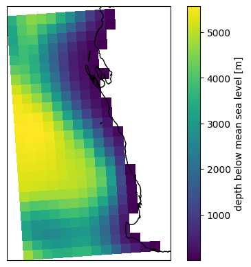
[41]:
fig, ax = plt.subplots(subplot_kw=dict(projection=ccrs.PlateCarree()))
p = dsgrid.depth.isel(time=0, drop=True).plot(ax=ax, x="longitude", y="latitude")
ax.coastlines();
Plot gridded Hs#
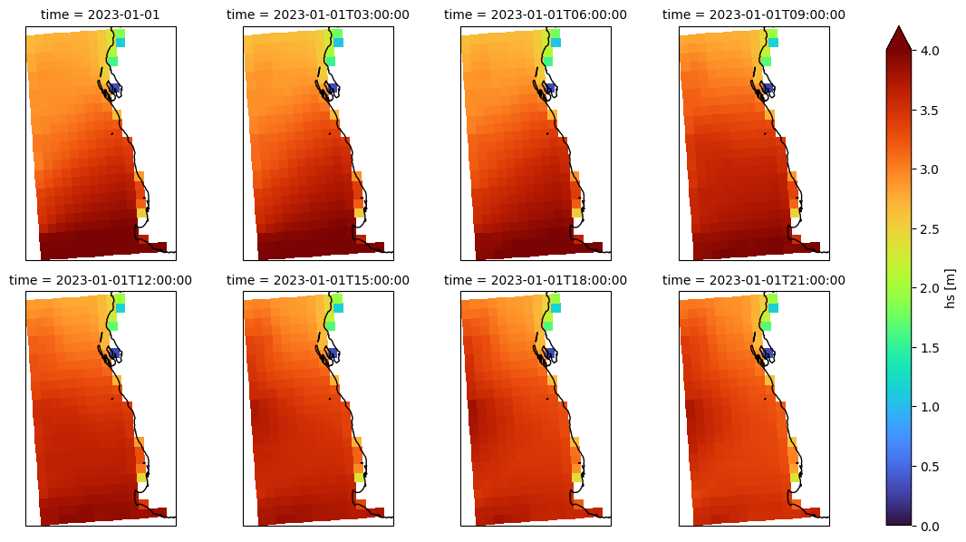
[42]:
f = dsgrid.hs.isel(time=slice(0, -1, 3)).plot(
    x="longitude",
    y="latitude",
    col="time",
    col_wrap=4,
    vmin=0,
    vmax=4,
    cmap="turbo",
    subplot_kws=dict(projection=ccrs.PlateCarree()),
)
f.map(lambda: plt.gca().coastlines());
Plot gridded wind#
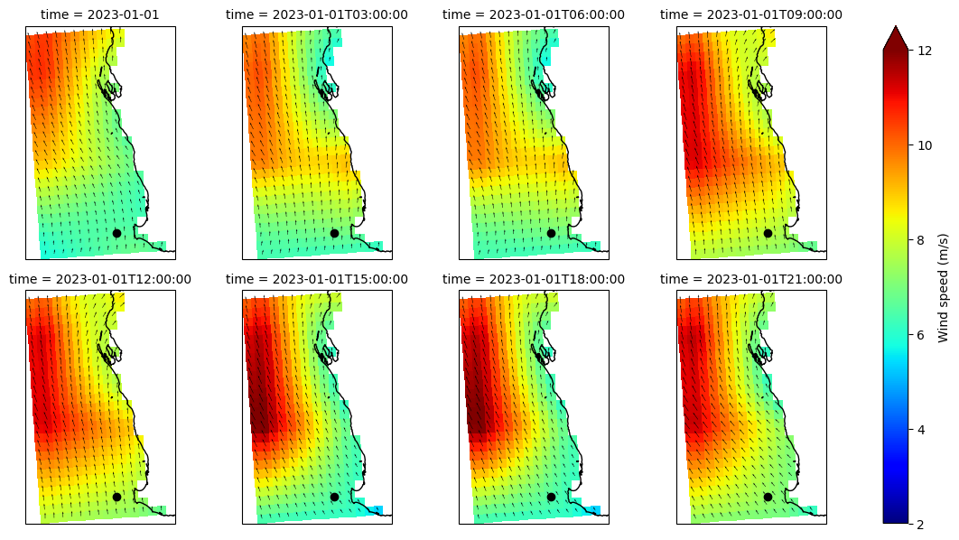
[43]:
u = dsgrid.xwnd.isel(time=slice(0, -1, 3))
v = dsgrid.ywnd.isel(time=slice(0, -1, 3))
f = np.sqrt(u ** 2 + v ** 2).plot(
    x="longitude",
    y="latitude",
    col="time",
    col_wrap=4,
    vmin=2,
    vmax=12,
    cmap="jet",
    cbar_kwargs={"label": "Wind speed (m/s)"},
    subplot_kws=dict(projection=ccrs.PlateCarree()),
)
for ax, time in zip(f.axs.flat, u.time):
    ax.coastlines()
    ax.quiver(u.longitude, u.latitude, u.sel(time=time), v.sel(time=time), scale=200)
    ax.plot(dspec.isel(site=0).lon, dspec.isel(site=0).lat, "ok")
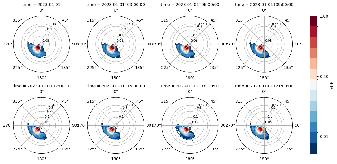
Plot spectra#
[44]:
p = dspec.isel(site=0, time=slice(0, -1, 3)).spec.plot(col="time", col_wrap=4)
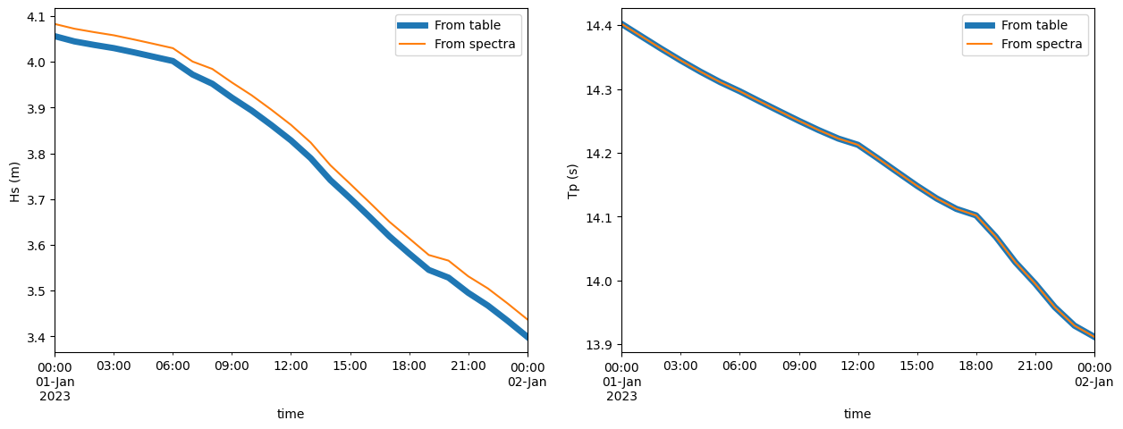
Plot timeseries#
[45]:
fig, (ax1, ax2) = plt.subplots(1, 2, figsize=(15, 5))

df.Hsig.plot(ax=ax1, label="From table", linewidth=5)
dspec.isel(site=0).spec.hs().to_pandas().plot(ax=ax1, label="From spectra")
ax1.set_ylabel("Hs (m)")
l = ax1.legend()

df.TPsmoo.plot(ax=ax2, label="From table", linewidth=5)
dspec.isel(site=0).spec.tp(smooth=True).to_pandas().plot(ax=ax2, label="From spectra")
ax2.set_ylabel("Tp (s)")
l = ax2.legend()
Plot hotfile#
[46]:
hotfiles = sorted(modeldir.glob(f"{run.config.lockup.compute.hotfile.fname.stem}*"))
hotfiles
[46]:
[PosixPath('example_procedural/run1/hotfile_20230101T010000.swn'),
 PosixPath('example_procedural/run1/hotfile_20230102T000000.swn')]
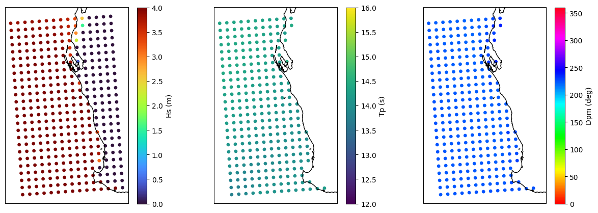
[47]:
# Investigate why the option to read as grid doesn't work

dset = read_swan(str(hotfiles[-1]), as_site=False)
stats = dset.spec.stats(["hs", "tp", "dpm"]).chunk()

fig, [ax1, ax2, ax3] = plt.subplots(1, 3, figsize=(15, 5), subplot_kw=dict(projection=ccrs.PlateCarree()))
p = ax1.scatter(dset.lon, dset.lat, s=15, c=stats.hs, vmin=0, vmax=4, cmap="turbo")
plt.colorbar(p, label="Hs (m)")
p = ax2.scatter(dset.lon, dset.lat, s=15, c=stats.tp, vmin=12, vmax=16, cmap="viridis")
plt.colorbar(p, label="Tp (s)")
p = ax3.scatter(dset.lon, dset.lat, s=15, c=stats.dpm, vmin=0, vmax=360, cmap="hsv")
plt.colorbar(p, label="Dpm (deg)")
for ax in [ax1, ax2, ax3]:
    ax.coastlines();