XBeach regular grid¶

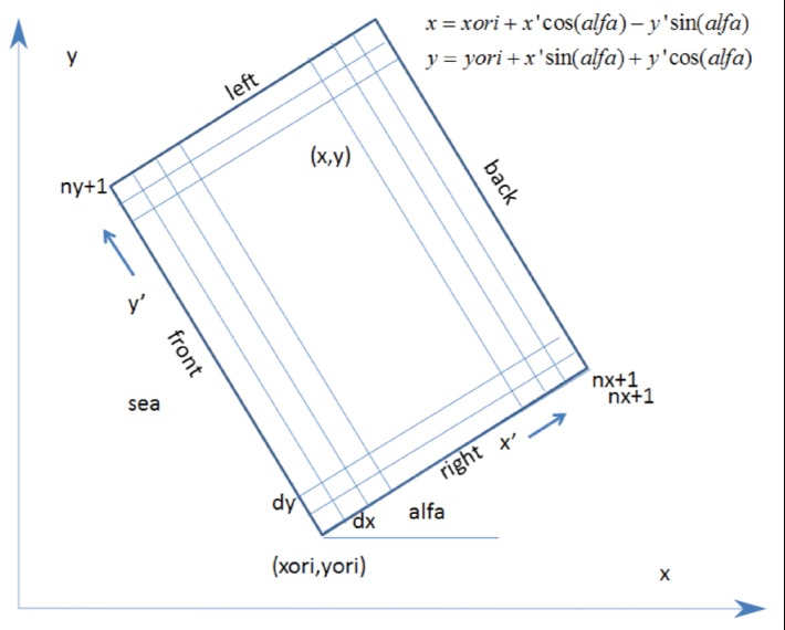
Usage demo for the XBeach RegularGrid object (image modified from the xbeach docs)

Requirements¶

• Clone and install the main version of rompy-xbeach
• The OSM land plot requires datamesh token to query the OSM land polygon but it is only for demonstration purposes

In [1]:

%load_ext autoreload
%autoreload 2

%load_ext autoreload %autoreload 2

In [2]:

import matplotlib.pyplot as plt
import cartopy.crs as ccrs
import cartopy.feature as cfeature
import geopandas
from shapely.geometry import shape

from rompy_xbeach.grid import GeoPoint, RegularGrid

import warnings
warnings.filterwarnings("ignore")

import matplotlib.pyplot as plt import cartopy.crs as ccrs import cartopy.feature as cfeature import geopandas from shapely.geometry import shape from rompy_xbeach.grid import GeoPoint, RegularGrid import warnings warnings.filterwarnings("ignore")

Grid origin¶

The origin of the RegularGrid is defined using the GeoPoint object which holds the coordinates of the origin x, y and the crs in which the coordinates are defined, allowing to define the origin in different coordinate systems such as WGS84 or projected coordinates

In [3]:

ori = GeoPoint(x=115.5875, y=-32.646, crs=4326)
ori

ori = GeoPoint(x=115.5875, y=-32.646, crs=4326) ori

Out[3]:

GeoPoint(x=115.5875, y=-32.646, crs='EPSG:4326')

A GeoPoint instance can be reprojected

In [4]:

ori_projected = ori.reproject(28350)
ori_projected

ori_projected = ori.reproject(28350) ori_projected

Out[4]:

GeoPoint(x=367520.0758689749, y=6387075.392325714, crs='EPSG:28350')

In [5]:

ori_projected.reproject(4326)

ori_projected.reproject(4326)

Out[5]:

GeoPoint(x=115.58749999999999, y=-32.646, crs='EPSG:4326')

Create the grid¶

The other parameters to construct the grid are similar to the other regular grid objects in rompy with the inclusion of the field crs to define the coordinate reference system of the xbeach grid. Note the origin coordinates can be prescribed in any known coordinate system

In [6]:

grid = RegularGrid(
    ori=GeoPoint(x=115.5875, y=-32.646, crs="epsg:4326"),
    alfa=344.0,
    dx=10,
    dy=20,
    nx=270,
    ny=305,
    crs="28350",
)
grid

grid = RegularGrid( ori=GeoPoint(x=115.5875, y=-32.646, crs="epsg:4326"), alfa=344.0, dx=10, dy=20, nx=270, ny=305, crs="28350", ) grid

Out[6]:

RegularGrid(ori=GeoPoint(x=115.5875, y=-32.646, crs='EPSG:4326'), alfa=344.0, dx=10.0, dy=20.0, nx=270, ny=305, crs='EPSG:28350')

Grid attributes¶

Some of the attributes of an XBeach grid instance include:¶

Projected origin coordinates

In [7]:

# The x0, y0 properties are the coordinates of the origin in the grid's crs
# (regardless of the crs defined in Ori)

grid.x0, grid.y0

# The x0, y0 properties are the coordinates of the origin in the grid's crs # (regardless of the crs defined in Ori) grid.x0, grid.y0

Out[7]:

(367520.0758689749, 6387075.392325714)

Centre of the offshore boundary

In [8]:

grid.offshore

grid.offshore

Out[8]:

(368358.01343065855, 6389997.627881368)

Centre of the grid

In [9]:

grid.centre

grid.centre

Out[9]:

(369650.91041169566, 6389626.895637793)

Grid shape

In [10]:

grid.shape

grid.shape

Out[10]:

(305, 270)

Stereographic projection

In [11]:

# A stereographic projection centered on the origin of the grid

grid.projection

# A stereographic projection centered on the origin of the grid grid.projection

Out[11]:

<cartopy.crs.Stereographic object at 0x74a8b6707800>

Cartopy transform

In [12]:

# The cartopy transform to reference the grid data when plotting

grid.transform

# The cartopy transform to reference the grid data when plotting grid.transform

Out[12]:

<cartopy._epsg._EPSGProjection object at 0x74a8b6707950>

Grid GeoDataFrame

In [13]:

# A MultiPolygon geometry representing each cell in the grid

grid.gdf

# A MultiPolygon geometry representing each cell in the grid grid.gdf

Out[13]:

	geometry	Name
0	MULTIPOLYGON (((367520.076 6387075.392, 367529...	{'grid_type': 'base', 'model_type': 'regular',...

Coordinates of the different sides

In [14]:

# Tuples of the (x, y) coordinates of each grid side. Uncomment to visualise

# grid.front
# grid.back
# grid.left
# grid.right

# Tuples of the (x, y) coordinates of each grid side. Uncomment to visualise # grid.front # grid.back # grid.left # grid.right

Plot the grid¶

A plotting method has been defined to allow dealing with different crs and projections. The offshore boundary and the grid origin are overlaid by default to help positioning the grid correctly

In [15]:

ax = grid.plot()

ax = grid.plot()

Coastlines¶

The coastlines from the GSHHS database are used which can be slower to plot but are considerably more detailed than the "10m" resolution version used by default in Cartopy

In [16]:

# Coastlines are defined by specifying the GSHHS resolution

ax = grid.plot(scale="f")

# Coastlines are defined by specifying the GSHHS resolution ax = grid.plot(scale="f")

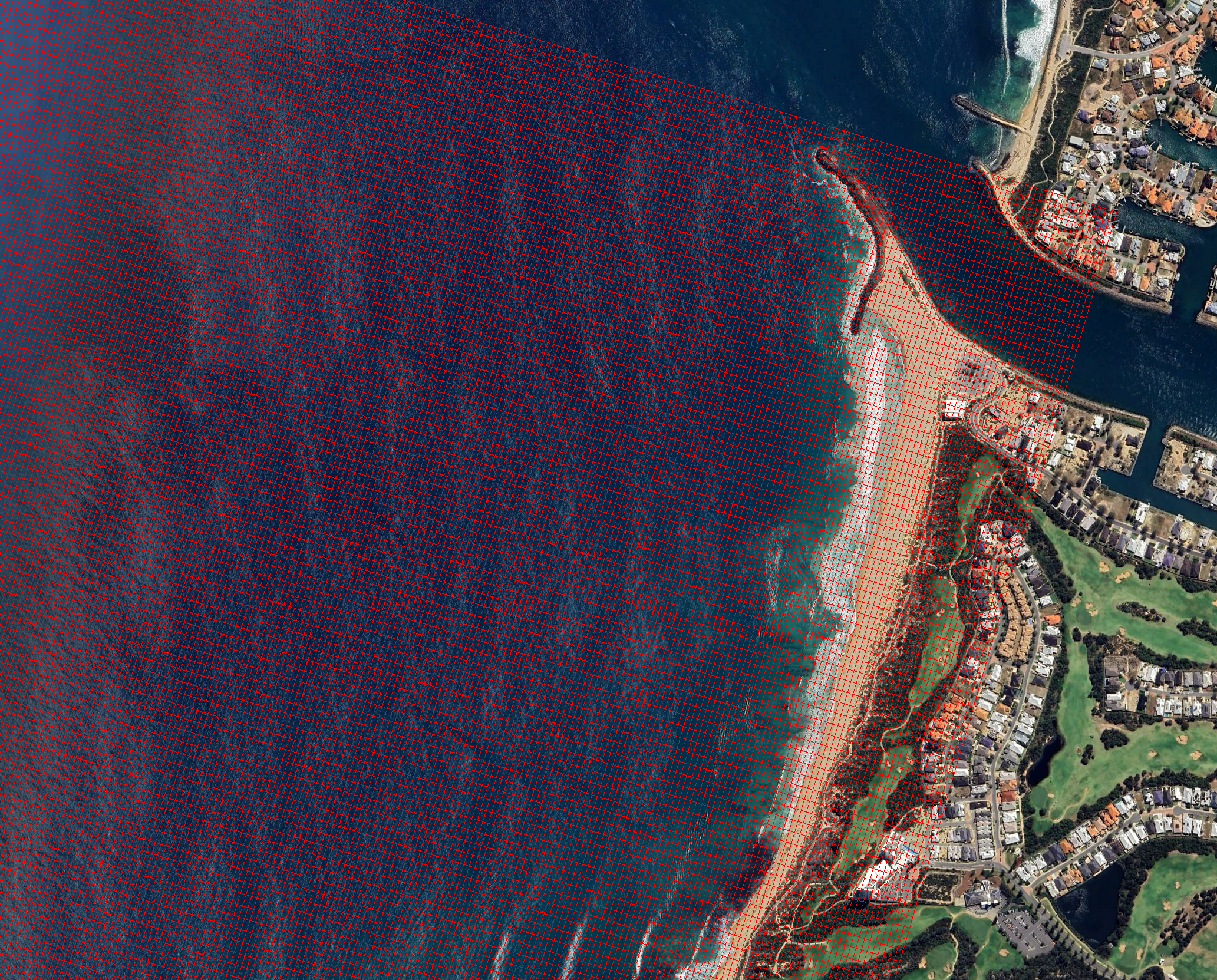
Grid mesh¶

The grid mesh can be overlaid

In [17]:

# The full mesh is shown by default but they can be downsampled for better visualisation

ax = grid.plot(scale="i", show_mesh=True, mesh_step=10)

# The full mesh is shown by default but they can be downsampled for better visualisation ax = grid.plot(scale="i", show_mesh=True, mesh_step=10)

In [18]:

# The appearance of the mesh can be customised using standard matplotlib parameters

ax = grid.plot(
    scale="i",
    show_mesh=True,
    mesh_step=20,
    mesh_kwargs=dict(color="red", alpha=0.5, linewidth=1.0),
)

# The appearance of the mesh can be customised using standard matplotlib parameters ax = grid.plot( scale="i", show_mesh=True, mesh_step=20, mesh_kwargs=dict(color="red", alpha=0.5, linewidth=1.0), )

Grid boundaries¶

The offshore boundary is highlighted by default but all boundaries can explicitly overlaid

In [19]:

# Plot a transparent grid without the origin and offshore side highlighted
ax = grid.plot(
    scale="f",
    grid_kwargs=dict(facecolor="none"),
    show_origin=False,
    show_offshore=False,
)

# Use the grid attributes to plot each side of the grid
ax.plot(grid.front[0], grid.front[1], "c", transform=grid.transform, label="Front")
ax.plot(grid.left[0], grid.left[1], "r", transform=grid.transform, label="Left")
ax.plot(grid.back[0], grid.back[1], "b", transform=grid.transform, label="Back")
ax.plot(grid.right[0], grid.right[1], "g", transform=grid.transform, label="Right")

l = ax.legend(loc="upper left")

# Plot a transparent grid without the origin and offshore side highlighted ax = grid.plot( scale="f", grid_kwargs=dict(facecolor="none"), show_origin=False, show_offshore=False, ) # Use the grid attributes to plot each side of the grid ax.plot(grid.front[0], grid.front[1], "c", transform=grid.transform, label="Front") ax.plot(grid.left[0], grid.left[1], "r", transform=grid.transform, label="Left") ax.plot(grid.back[0], grid.back[1], "b", transform=grid.transform, label="Back") ax.plot(grid.right[0], grid.right[1], "g", transform=grid.transform, label="Right") l = ax.legend(loc="upper left")

Projections¶

Cartopy projections are fully supported

In [20]:

# Use a PlateCarree projection

ax = grid.plot(
    scale="f",
    projection=ccrs.PlateCarree(),
    grid_kwargs=dict(alpha=0.5, facecolor="black", zorder=2),
)

# Use a PlateCarree projection ax = grid.plot( scale="f", projection=ccrs.PlateCarree(), grid_kwargs=dict(alpha=0.5, facecolor="black", zorder=2), )

Land masks¶

It is possible to use land masks other than the GSHHS ones. In the example below we are going to define an arbitrary a GeoDataFrame object with some land Polygon to exemplify it

In [21]:

def get_land_feature() -> geopandas.GeoDataFrame:
    """Generate GeoDataFrame with a Polygon feature representing the land."""
    feature = cfeature.NaturalEarthFeature(category="physical", name="land", scale="10m")
    return geopandas.GeoDataFrame(
        geometry=[shape(feature) for feature in feature.geometries()], crs="EPSG:4326"
    ).dissolve()


land = get_land_feature()
land

def get_land_feature() -> geopandas.GeoDataFrame: """Generate GeoDataFrame with a Polygon feature representing the land.""" feature = cfeature.NaturalEarthFeature(category="physical", name="land", scale="10m") return geopandas.GeoDataFrame( geometry=[shape(feature) for feature in feature.geometries()], crs="EPSG:4326" ).dissolve() land = get_land_feature() land

Out[21]:

	geometry
0	MULTIPOLYGON (((-170.84708 -83.00543, -171.339...

In [22]:

# Plot the grid initially without any land mask
ax = grid.plot(projection=ccrs.PlateCarree(), show_offshore=False)

# Plot the land mask separately
ax = land.plot(ax=ax, transform=ccrs.PlateCarree(), color="gray")

# Plot the grid initially without any land mask ax = grid.plot(projection=ccrs.PlateCarree(), show_offshore=False) # Plot the land mask separately ax = land.plot(ax=ax, transform=ccrs.PlateCarree(), color="gray")

Compare the different GSHHS coastline scales

In [23]:

fig, axs = plt.subplots(1, 5, figsize=(20, 4), subplot_kw=dict(projection=grid.projection))

resolution = {
    "crude": "c",
    "low": "l",
    "intermediate": "i",
    "high": "h",
    "full": "f",
}
for ax, (key, value) in zip(axs, resolution.items()):
    grid.plot(ax=ax, scale=value, buffer=5000)
    ax.set_title(key)

fig, axs = plt.subplots(1, 5, figsize=(20, 4), subplot_kw=dict(projection=grid.projection)) resolution = { "crude": "c", "low": "l", "intermediate": "i", "high": "h", "full": "f", } for ax, (key, value) in zip(axs, resolution.items()): grid.plot(ax=ax, scale=value, buffer=5000) ax.set_title(key)

Compare the different NaturalEarthFeature scales

In [24]:

fig, axs = plt.subplots(1, 3, figsize=(11, 3.5), subplot_kw=dict(projection=grid.projection))

for ax, scale in zip(axs, ["110m", "50m", "10m"]):
    ax.add_feature(cfeature.LAND.with_scale(scale), facecolor="0.7", edgecolor="0.3", linewidth=0.5)
    grid.plot(ax=ax, scale=None, buffer=5000)
    ax.set_title(scale)

fig, axs = plt.subplots(1, 3, figsize=(11, 3.5), subplot_kw=dict(projection=grid.projection)) for ax, scale in zip(axs, ["110m", "50m", "10m"]): ax.add_feature(cfeature.LAND.with_scale(scale), facecolor="0.7", edgecolor="0.3", linewidth=0.5) grid.plot(ax=ax, scale=None, buffer=5000) ax.set_title(scale)

Expand the grid¶

The grid can be expanded which is useful when extending the offshore and lateral boundaries

In [25]:

# Individual sides are expanded by a specified number of cells

grid_extended = grid.expand(left=5, right=5, front=30)

print(grid)
print(grid_extended)

# Individual sides are expanded by a specified number of cells grid_extended = grid.expand(left=5, right=5, front=30) print(grid) print(grid_extended)

RegularGrid(ori=GeoPoint(x=115.5875, y=-32.646, crs='EPSG:4326'), alfa=344.0, dx=10.0, dy=20.0, nx=270, ny=305, crs='EPSG:28350')
RegularGrid(ori=GeoPoint(x=115.58413040314187, y=-32.64608321400174, crs='EPSG:4326'), alfa=344.0, dx=10.0, dy=20.0, nx=300, ny=315, crs='EPSG:28350')

In [26]:

fig, ax = plt.subplots(figsize=(6, 6), subplot_kw=dict(projection=grid.projection))

grid_extended.plot(ax=ax, scale="i", grid_kwargs=dict(facecolor="y", edgecolor="k", alpha=0.5, zorder=2))
grid.plot(ax=ax, grid_kwargs=dict(facecolor="k", edgecolor="k", alpha=0.5, zorder=3))

fig, ax = plt.subplots(figsize=(6, 6), subplot_kw=dict(projection=grid.projection)) grid_extended.plot(ax=ax, scale="i", grid_kwargs=dict(facecolor="y", edgecolor="k", alpha=0.5, zorder=2)) grid.plot(ax=ax, grid_kwargs=dict(facecolor="k", edgecolor="k", alpha=0.5, zorder=3))

Out[26]:

<GeoAxes: >

Save the grid¶

A custom method is provided to save the grid as a MultiPolygon GeoDataFrame object which can be visualised on GIS software

In [27]:

grid.to_file("grid.kml", driver="KML")

grid.to_file("grid.kml", driver="KML")

2025-10-02 18:20:41 [INFO] pyogrio._io         : Created 1 records

Open and visualise it on GGE

Alternatively, a GeoDataFrame of the grid boundaries can be defined and saved to file (which can be useful if the grid is too large)

In [28]:

import geopandas as gpd

gdf = gpd.GeoSeries(grid.boundary(), crs=grid.crs)
gdf.to_file("grid_boundaries.kml", driver="KML")

import geopandas as gpd gdf = gpd.GeoSeries(grid.boundary(), crs=grid.crs) gdf.to_file("grid_boundaries.kml", driver="KML")

2025-10-02 18:20:41 [INFO] pyogrio._io         : Created 1 records

Recreate the grid¶

The (full) grid file also stores some grid metadata to allow recreating a grid object (making it easy to share)

In [29]:

grid2 = RegularGrid.from_file("grid.kml")
grid2.plot(scale="i")

grid2 = RegularGrid.from_file("grid.kml") grid2.plot(scale="i")

Out[29]:

<GeoAxes: >