2. Defining the model grid¶

What this shows: how to place, rotate and size an XBeach grid with RegularGrid, and how to check it is oriented correctly.

Prerequisites: 1. Your first XBeach model.

You will learn:

• how GeoPoint handles coordinates in different reference systems
• what ori, alfa, dx, dy, nx, ny and crs mean
• the XBeach orientation convention: offshore boundary, origin and axes
• how to inspect grid geometry and extend a grid

Data used: none.

Setup¶

In [1]:

import matplotlib.pyplot as plt
from rompy_xbeach.grid import GeoPoint, RegularGrid

import matplotlib.pyplot as plt from rompy_xbeach.grid import GeoPoint, RegularGrid

1. Points with a coordinate reference system¶

A GeoPoint is a coordinate pair plus its CRS. It can be reprojected, so you can give the grid origin in whatever system your data uses.

In [2]:

origin = GeoPoint(x=115.594239, y=-32.641104, crs=4326)
origin_mga = origin.reproject(28350)
print(f"WGS84:        x={origin.x:.6f}, y={origin.y:.6f}")
print(f"MGA zone 50:  x={origin_mga.x:.1f}, y={origin_mga.y:.1f}")

origin = GeoPoint(x=115.594239, y=-32.641104, crs=4326) origin_mga = origin.reproject(28350) print(f"WGS84: x={origin.x:.6f}, y={origin.y:.6f}") print(f"MGA zone 50: x={origin_mga.x:.1f}, y={origin_mga.y:.1f}")

WGS84:        x=115.594239, y=-32.641104
MGA zone 50:  x=368145.0, y=6387626.6

2. The grid definition¶

XBeach uses a rectilinear grid whose x-axis runs cross-shore, from the offshore boundary towards land:

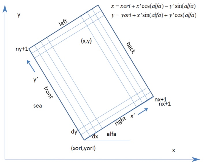
Adapted from the XBeach manual.

Field	Meaning
ori	Origin, the corner of the grid on the offshore boundary
alfa	Angle of the x-axis, degrees counter-clockwise from east
dx, dy	Cell size along x (cross-shore) and y (alongshore), in crs units
nx, ny	Number of grid points along x and y
crs	Projected CRS the grid is built in (metres)

On this west-facing coast the x-axis must point roughly east, so alfa=347 rotates it 13° clockwise from east.

In [3]:

grid = RegularGrid(
    ori=origin,
    alfa=347.0,
    dx=10.0,
    dy=15.0,
    nx=230,
    ny=220,
    crs=28350,
)
grid

grid = RegularGrid( ori=origin, alfa=347.0, dx=10.0, dy=15.0, nx=230, ny=220, crs=28350, ) grid

Out[3]:

RegularGrid(ori=GeoPoint(x=115.594239, y=-32.641104, crs='EPSG:4326'), alfa=347.0, dx=10.0, dy=15.0, nx=230, ny=220, crs='EPSG:28350')

3. Checking the orientation¶

plot() marks the origin (red dot) and the offshore boundary (red line). The offshore boundary must face the open sea.

In [4]:

ax = grid.plot(scale="f")

ax = grid.plot(scale="f")

Each side of the grid has a name used by XBeach boundary conditions: front is offshore, back is landward, and left and right are the lateral sides.

In [5]:

ax = grid.plot(
    scale="f", grid_kwargs={"facecolor": "none"}, show_origin=False, show_offshore=False
)
for side, colour in [
    ("front", "red"),
    ("back", "blue"),
    ("left", "orange"),
    ("right", "green"),
]:
    ax.plot(
        *getattr(grid, side),
        color=colour,
        linewidth=3,
        transform=grid.transform,
        label=side,
    )
ax.legend(loc="upper left")

ax = grid.plot( scale="f", grid_kwargs={"facecolor": "none"}, show_origin=False, show_offshore=False ) for side, colour in [ ("front", "red"), ("back", "blue"), ("left", "orange"), ("right", "green"), ]: ax.plot( *getattr(grid, side), color=colour, linewidth=3, transform=grid.transform, label=side, ) ax.legend(loc="upper left")

Out[5]:

<matplotlib.legend.Legend at 0x71062f9072c0>

A common mistake¶

Putting the origin on the landward side, with the axis flipped, gives a grid that covers the same area but has its offshore boundary on land. XBeach would force waves from the beach.

In [6]:

wrong = RegularGrid(
    ori=GeoPoint(x=grid.x[-1, -1], y=grid.y[-1, -1], crs=grid.crs),
    alfa=grid.alfa - 180,
    dx=grid.dx,
    dy=grid.dy,
    nx=grid.nx,
    ny=grid.ny,
    crs=grid.crs,
)
ax = wrong.plot(scale="f", grid_kwargs={"facecolor": "red", "alpha": 0.3, "zorder": 2})
ax.set_title("Wrong: offshore boundary on land")

wrong = RegularGrid( ori=GeoPoint(x=grid.x[-1, -1], y=grid.y[-1, -1], crs=grid.crs), alfa=grid.alfa - 180, dx=grid.dx, dy=grid.dy, nx=grid.nx, ny=grid.ny, crs=grid.crs, ) ax = wrong.plot(scale="f", grid_kwargs={"facecolor": "red", "alpha": 0.3, "zorder": 2}) ax.set_title("Wrong: offshore boundary on land")

Out[6]:

Text(0.5, 1.0, 'Wrong: offshore boundary on land')

4. Grid geometry¶

The grid exposes its geometry for plotting and for selecting forcing data. Forcing is usually taken at the centre of the grid or at the middle of the offshore boundary.

In [7]:

print(f"Origin in grid CRS: x0={grid.x0:.1f}, y0={grid.y0:.1f}")
print(f"Shape (ny, nx):     {grid.shape}")
print(f"Grid centre:        {grid.centre}")
print(f"Offshore midpoint:  {grid.offshore}")
print(f"Coordinate arrays:  x {grid.x.shape}, y {grid.y.shape}")

print(f"Origin in grid CRS: x0={grid.x0:.1f}, y0={grid.y0:.1f}") print(f"Shape (ny, nx): {grid.shape}") print(f"Grid centre: {grid.centre}") print(f"Offshore midpoint: {grid.offshore}") print(f"Coordinate arrays: x {grid.x.shape}, y {grid.y.shape}")

Origin in grid CRS: x0=368145.0, y0=6387626.6
Shape (ny, nx):     (220, 230)
Grid centre:        (369630.13818098354, 6388969.42314107)
Offshore midpoint:  (368514.48445680446, 6389226.992098292)
Coordinate arrays:  x (220, 230), y (220, 230)

5. The XBeach parameters¶

These are the values the grid contributes to params.txt. XBeach counts cells, so its nx and ny are one less than the number of grid points, and vardx=0 tells XBeach the grid has constant spacing.

In [8]:

for key, value in grid.params.items():
    print(f"{key} = {value}")

for key, value in grid.params.items(): print(f"{key} = {value}")

vardx = 0
nx = 229
ny = 219
dx = 10.0
dy = 15.0
xori = 368145.00235004467
yori = 6387626.589266883
alfa = 347.0
projection = +proj=utm +zone=50 +south +ellps=GRS80 +units=m +no_defs +type=crs

6. Extending a grid¶

expand() adds cells on any side. The bathymetry class uses it to extend the domain offshore and laterally (see Tutorial 3).

In [9]:

extended = grid.expand(front=30, left=10, right=10)
print(f"Original: {grid.nx} x {grid.ny} points")
print(f"Extended: {extended.nx} x {extended.ny} points")

fig, ax = plt.subplots(figsize=(6, 6), subplot_kw={"projection": grid.projection})
extended.plot(ax=ax, scale="i", grid_kwargs={"facecolor": "gold", "alpha": 0.5})
grid.plot(ax=ax, grid_kwargs={"facecolor": "black", "alpha": 0.4}, set_extent=False)
ax.set_title("Original (dark) and extended (gold) grid")

extended = grid.expand(front=30, left=10, right=10) print(f"Original: {grid.nx} x {grid.ny} points") print(f"Extended: {extended.nx} x {extended.ny} points") fig, ax = plt.subplots(figsize=(6, 6), subplot_kw={"projection": grid.projection}) extended.plot(ax=ax, scale="i", grid_kwargs={"facecolor": "gold", "alpha": 0.5}) grid.plot(ax=ax, grid_kwargs={"facecolor": "black", "alpha": 0.4}, set_extent=False) ax.set_title("Original (dark) and extended (gold) grid")

Original: 230 x 220 points
Extended: 260 x 240 points

Out[9]:

Text(0.5, 1.0, 'Original (dark) and extended (gold) grid')

Summary¶

• The grid origin sits on the offshore boundary, and the x-axis points towards land.
• alfa is measured counter-clockwise from east.
• Always plot a new grid and check that the red offshore boundary faces the sea.

Next: 3. Bathymetry from your data.

See also: Grid plotting and export covers coastline options, projections and saving grids to KML or GeoJSON.

---

Previous lesson: notebooks-xbeach-tutorial-01-first-model · Next lesson: notebooks-xbeach-tutorial-03-bathymetry